Transformer Architecture

The Transformer is a neural network for sequences that replaces recurrence with attention. Instead of reading words one by one like an RNN, it looks at all the words of a sentence at the same time and learns which words are relevant to each other. This removes the sequential bottleneck of RNNs and makes training much faster on modern hardware. This page walks through the architecture part by part: input, positional encoding, encoder, shifted output, decoder, output layer, the attention mechanism, two training tricks (multi-head attention and label smoothing), and the input and output shapes of cross-attention.

The Transformer has two stacks: an encoder that reads the input sequence and a decoder that produces the output sequence one token at a time. Each stack is built from three kinds of components. The attention layer (multi-head attention, MHA) lets every token gather information from other tokens. The feed forward neural network (FFNN) then processes each token's vector further. Positional encoding (PE) is added at the start, because attention by itself has no sense of word order.

Attention is used in three ways: self-attention in the encoder (encoder-encoder), masked self-attention in the decoder (decoder-decoder), and an encoder-decoder attention layer that lets the decoder look at the encoder's output.

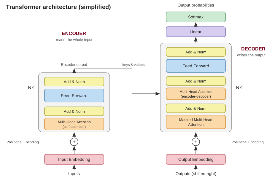
Task: translate "I love cats" (English) -> "Ich liebe Katzen" (German)

Encoder          : reads "I love cats" and builds a rich vector for each word
Decoder          : writes "Ich", then "liebe", then "Katzen", one at a time
Encoder-decoder
attention        : while writing "Katzen", the decoder looks back at "cats"
    

The input text is first tokenized into tokens (words or subwords), and each token is mapped to an integer ID from a vocabulary of size V. The ID selects one row of a learned embedding matrix, which turns the token into a vector of d_model numbers. These embeddings are learned during training, just like the embeddings in Word2vec, so tokens with similar meaning end up with similar vectors. The result is one d_model-sized vector per token, which is what the rest of the network works with.

Text      : "The cat sat"
Tokens    : ["The", "cat", "sat"]
Token IDs : [12, 87, 45]                       (illustrative IDs)
Embedding : each ID -> a row of the V x d_model matrix
            "The" -> [0.12, -0.40, ..., 0.05]  (d_model numbers)
            "cat" -> [0.33,  0.18, ..., -0.21]
            "sat" -> [-0.07, 0.25, ..., 0.44]

If V = 30,000 and d_model = 512, the matrix has 30,000 x 512 = 15.36 million values.
    

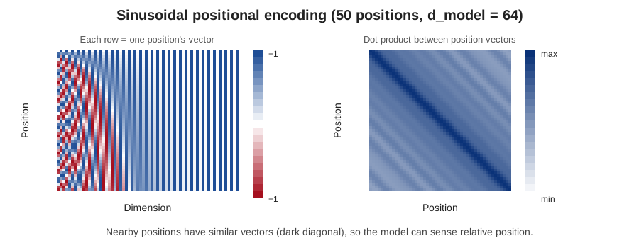
Attention looks at all tokens at once, so without extra information the model would see "dog bites man" and "man bites dog" as the same bag of words. Positional encoding fixes this by adding a position-dependent vector to each token embedding. These vectors can be learned, or hardcoded with sine and cosine waves of different frequencies, as in the original paper. The goal is to let the model understand the relative position of tokens: in the right-hand picture, positions that are close together have a higher dot product than positions that are far apart.

The sinusoidal version is:

\(PE_{(pos,\,2i)} = \sin\left(\dfrac{pos}{10000^{2i/d_{model}}}\right)\),   \(PE_{(pos,\,2i+1)} = \cos\left(\dfrac{pos}{10000^{2i/d_{model}}}\right)\)

d_model = 4. The vector added to the embedding at each position:

pos 0: [ 0.000,  1.000, 0.000, 1.000]
pos 1: [ 0.841,  0.540, 0.010, 1.000]
pos 2: [ 0.909, -0.416, 0.020, 1.000]

Final input of a token = token embedding + positional encoding
So "cat" at position 1 and "cat" at position 5 get different input vectors.
    

The encoder is a stack of N identical layers. Each layer has two sub-layers: encoder-encoder (self-)attention, where every token looks at all other input tokens, and a feed forward neural network that is applied to each token separately. After each sub-layer there is an Add & Norm step: the sub-layer's input is added back to its output (a residual connection) and the result is normalized, which keeps training stable in deep stacks. The final output is a context-aware vector for every input token.

N is the number of stacked layers and h is the number of attention heads. d_FF is the hidden size of the feed forward network, d_key and d_value are the sizes of the key and value vectors in attention, and d_model is the embedding size. The original paper's base model used N = 6, h = 8, d_model = 512, d_FF = 2048 and d_key = d_value = 64.

Input : "I love cats"  (3 token vectors + positional encoding)

Layer 1, self-attention : "love" gathers information from "I" and "cats"
Layer 1, Add & Norm     : output = LayerNorm(input + attention output)
Layer 1, Feed Forward   : each of the 3 vectors is transformed independently
Layer 1, Add & Norm     : output = LayerNorm(input + FFNN output)
... repeated N times ...
Output: 3 context-aware vectors, passed to the decoder
    

The decoder's input is the target sentence, embedded with its own learned embeddings (of size d_model, over a vocabulary of size V) plus positional encoding. It is "shifted right" by one position: a special start token [BOS] is placed at the front and the last word is dropped. As a result, at every position the decoder only sees the words that come before the one it must predict. In practice, translation starts from [BOS] alone, and each newly generated word is fed back in for the next step.

Target sentence : Ich   liebe   Katzen   [EOS]

Decoder input   : [BOS]  Ich     liebe    Katzen      (shifted right)
Expected output : Ich    liebe   Katzen   [EOS]

At position 1 the decoder sees only "[BOS]" and must predict "Ich".
At position 3 it sees "[BOS] Ich liebe" and must predict "Katzen".
    

The decoder is also a stack of N layers, but each layer has three sub-layers. First comes decoder-decoder (masked self-)attention, where each position can look only at earlier output positions, never at future ones. Then encoder-decoder attention lets the decoder look at the encoder's output: its queries come from the decoder, while its keys and values come from the encoder. Finally a feed forward network processes each position, and every sub-layer is followed by Add & Norm. The parameters are the same as in the encoder.

The mask matters because during training the whole target sentence is given at once. Without it, the decoder could simply copy the next word instead of learning to predict it.

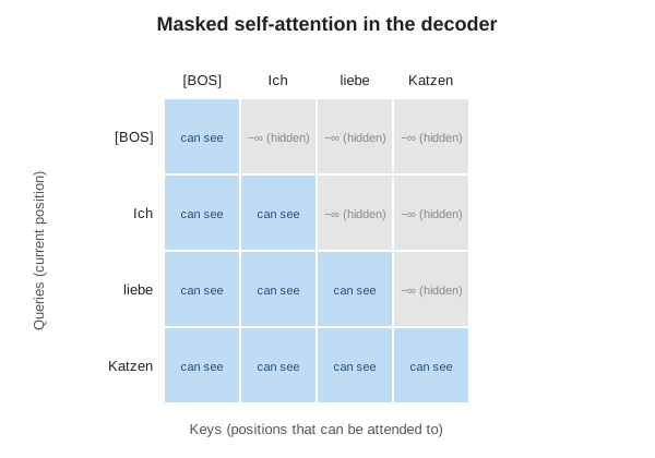
Decoder input: [BOS] Ich liebe Katzen

Masked self-attention : "liebe" may attend to [BOS], Ich, liebe  (not to Katzen)
Encoder-decoder attn  : while predicting "Katzen", attention is strongest
                        on the encoder vector for "cats"
Feed Forward + Norm   : refine each position's vector
    

The last decoder vector for each position has d_model numbers. A linear projection maps it to V numbers, one score for every word in the vocabulary. A softmax then turns these scores into probabilities that add up to 1. This is a classification problem in which each class is a word, so the model outputs the probability of each word being the next one, and the most likely word (or a sampled one) is chosen.

Vocabulary (V = 5): [Katzen, Hunde, Autos, Bäume, Himmel]

Linear scores : [3.2, 1.1, 0.3, -0.5, 0.2]
Softmax       : [0.80, 0.10, 0.04, 0.02, 0.04]   (sum = 1)

Predicted next word: "Katzen" (probability 0.80)
    

Each token produces three vectors: a query Q (what it is looking for), a key K (what it offers), and a value V (the information it passes on). The dot product of a query with every key gives a score for how relevant each token is, and dividing by \(\sqrt{d_k}\) keeps the scores from growing too large, which would make the softmax too sharp. An optional mask hides some positions (used in the decoder), the softmax turns the scores into weights that sum to 1, and the output is the weighted sum of the values. Because all of this is written as matrix multiplications, every token is processed at once on a GPU.

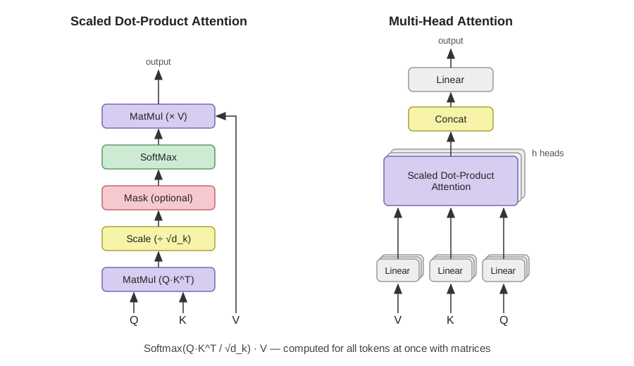
3 tokens, d_k = 2
Q = K = [[1,0],[0,1],[1,1]]      V = [[1,0],[0,2],[1,1]]

For token 1 (query [1,0]):
  scores Q.K^T         = [1, 0, 1]
  scaled (divide by 1.414) = [0.71, 0.00, 0.71]
  softmax weights      = [0.40, 0.20, 0.40]
  output = 0.40*[1,0] + 0.20*[0,2] + 0.40*[1,1] = [0.80, 0.80]

Token 1 pays equal attention to tokens 1 and 3, and less to token 2.
    

Instead of one attention operation, multi-head attention runs h of them in parallel (the right side of the figure above). Each head has its own learned linear projections of Q, K and V into smaller vectors, applies scaled dot-product attention, and the results of all heads are concatenated and passed through a final linear layer. This lets the model capture different kinds of relationships at the same time. It is comparable to the multiple filters of a convolutional layer in computer vision, where each filter detects a different pattern.

d_model = 512, h = 8 heads  ->  each head works with d_k = 512 / 8 = 64

Sentence: "The animal didn't cross the street because it was tired"

Head 1 might link  "it"      -> "animal"      (what "it" refers to)
Head 2 might link  "cross"   -> "street"      (verb and its object)
Head 3 might link  "tired"   -> "it"          (adjective and subject)

Heads learn their roles during training; these roles are only illustrations.
Concat(head 1 ... head 8) -> Linear -> one d_model vector per token
    

Normally the training target is a hard one-hot label: probability 1 for the correct word and 0 for all others. A 2015 vision paper showed that this encourages overconfidence, which is bad for generalization. Label smoothing introduces noise in the true labels by moving a small amount \(\epsilon\) of the probability mass onto all words, using a uniform distribution \(u(k) = 1/V\):

\(q(k|x) = \delta_{k,y} \;\longrightarrow\; q'(k|x) = (1-\epsilon)\,\delta_{k,y} + \epsilon\,u(k)\)

It is a general technique that prevents overfitting, and in the Transformer it improves accuracy and the BLEU score (a measure of how close a machine translation is to a human reference). The original paper also notes that it makes perplexity worse, because the model learns to be less certain.

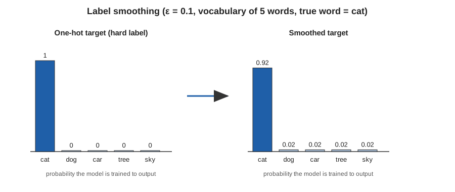
V = 5 words, true word = "cat", epsilon = 0.1, u(k) = 1/5 = 0.2

true word  : (1 - 0.1) * 1 + 0.1 * 0.2 = 0.90 + 0.02 = 0.92
other words: (1 - 0.1) * 0 + 0.1 * 0.2 = 0.00 + 0.02 = 0.02

One-hot target : [1.00, 0.00, 0.00, 0.00, 0.00]
Smoothed target: [0.92, 0.02, 0.02, 0.02, 0.02]   (still sums to 1)
    

In cross-attention, the queries come from one sequence (for example, the decoder) and the keys and values come from another sequence (for example, the encoder). Suppose there are N query vectors and M key vectors with M matching value vectors, all of dimension D. The scores \(QK^T\) form an N × M matrix, because every query is compared with every key. After the softmax, each row holds the weights of one query over the M keys and sums to 1. Multiplying this N × M weight matrix by the M × D value matrix gives an N × D output.

So the number of output tokens is N, the number of queries, and not M. Each query produces exactly one output vector, which is a weighted mix of all M value vectors. The number of keys and values M only decides how many items each query can choose from, and how large the score matrix is. (If the value vectors had a different size \(d_v\), the outputs would have dimension \(d_v\) instead of D.)

\(\underbrace{\text{softmax}\left(\dfrac{Q K^T}{\sqrt{D}}\right)}_{N \times M} \; \underbrace{V}_{M \times D} \;=\; \underbrace{\text{Output}}_{N \times D}\)

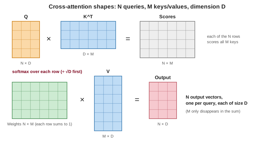
Translation: encoder reads "I love cats" -> M = 3 key/value vectors
             decoder has written "[BOS] Ich liebe Katzen" -> N = 4 query vectors
Result: N = 4 output vectors (one for each decoder position), no matter that M = 3.

Small numeric case: N = 2 queries, M = 3 keys/values, D = 2
Q = [[1,0],[0,1]]                 (2 x 2)
K = [[1,0],[0,1],[1,1]]           (3 x 2)
V = [[1,0],[0,2],[1,1]]           (3 x 2)

Scores Q.K^T / sqrt(2)  (2 x 3):
  query 1: [0.71, 0.00, 0.71]
  query 2: [0.00, 0.71, 0.71]
Softmax weights (2 x 3), each row sums to 1:
  query 1: [0.40, 0.20, 0.40]
  query 2: [0.20, 0.40, 0.40]
Output = weights x V  (2 x 2):
  query 1: 0.40*[1,0] + 0.20*[0,2] + 0.40*[1,1] = [0.80, 0.80]
  query 2: 0.20*[1,0] + 0.40*[0,2] + 0.40*[1,1] = [0.60, 1.20]

2 queries in -> 2 output vectors out, each of size D = 2.
If M grows from 3 to 100, the output is still 2 vectors of size 2.