
Mixture of Experts and Guided Decoding
Mixture of Experts and Guided Decoding
OverviewThis page covers two ideas that matter when building and using large language models. Mixture of Experts (MoE) makes a model larger without making every token more expensive, by sending each token only to a few specialist sub-networks. Guided decoding controls what the model is allowed to write, so that its output always follows a required format such as JSON. Between them sits sampling, the step where the next token is drawn from the model's probability distribution and where the format rules are enforced.
1. Mixture of Experts (MoE)
ConceptAn MoE layer replaces one big network with several smaller networks called experts, plus a gate (router) that decides how much each expert should contribute for a given input. The gate looks at the input \(x\) and produces one weight \(G(x)_i\) per expert. The final output \(\hat{y}\) is the weighted sum of the expert outputs \(E_i(x)\). In a Transformer, the experts are usually the feed forward networks, so an MoE layer takes the place of the feed forward block, while attention stays shared. The routing is done separately for every token.
3 experts, one input x, scalar outputs to keep the numbers simple

Gate weights    G(x) = [0.5, 0.3, 0.2]
Expert outputs  E(x) = [2.0, 4.0, 0.0]

y_hat = 0.5 * 2.0 + 0.3 * 4.0 + 0.2 * 0.0 = 1.0 + 1.2 + 0.0 = 2.2
2. Dense MoE
VariantIn a dense MoE, the gate gives a non-zero weight to every expert, usually with a softmax over all of them, and every expert is run for every token. The output is a smooth blend of all experts, and the formula is exactly the one above with all n terms. This is easy to train, because every expert receives a learning signal from every token. The drawback is cost: the compute grows with the number of experts, so adding experts makes the model slower and does not give the efficiency benefit that MoE is known for.
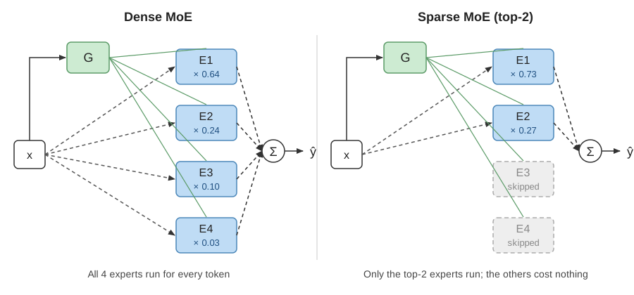
4 experts, gate scores (logits) = [2.0, 1.0, 0.1, -1.0]

Softmax over all 4 : [0.64, 0.24, 0.10, 0.03]   (all experts get a weight)
Experts run        : E1, E2, E3, E4              (4 experts of compute)
3. Sparse MoE
VariantA sparse MoE keeps only the top-k gate scores for each token, applies the softmax over those k scores, and gives every other expert a weight of exactly 0. Experts with weight 0 are simply not run. This breaks the link between model size and cost: the model can hold many experts (many parameters), but each token pays only for k of them. For example, Mixtral 8x7B has 8 experts per layer and picks the top 2 for each token, so it has about 47 billion parameters in total but uses only about 13 billion of them per token. The price is extra complexity in training, shown in the next section.
import torch
import torch.nn as nn

class SparseMoE(nn.Module):
    def __init__(self, experts, d_model, top_k=2):
        super().__init__()
        self.experts = nn.ModuleList(experts)
        self.gate = nn.Linear(d_model, len(experts), bias=False)
        self.top_k = top_k

    def forward(self, x):                              # x: (num_tokens, d_model)
        logits = self.gate(x)                          # one score per expert
        weights, chosen = torch.topk(logits, self.top_k, dim=-1)
        weights = torch.softmax(weights, dim=-1)       # softmax over the chosen experts only
        out = torch.zeros_like(x)
        for i, expert in enumerate(self.experts):
            token_idx, slot = torch.where(chosen == i) # tokens that selected expert i
            if token_idx.numel() == 0:
                continue                               # expert i is skipped entirely
            out[token_idx] += weights[token_idx, slot, None] * expert(x[token_idx])
        return out
Same gate scores as before: [2.0, 1.0, 0.1, -1.0], top-2 routing

Top-2 experts  : E1 (2.0) and E2 (1.0)
Softmax on those two : [0.73, 0.27]
Final weights  : [0.73, 0.27, 0, 0]       (E3 and E4 are not computed)

Dense vs sparse
                     Dense MoE            Sparse MoE
Gate weights         all non-zero         only k non-zero
Experts run / token  n                    k
Parameters           all used each time   many, but few used each time
Training             simple               needs load balancing
4. Training Challenge: Routing Collapse
TrainingIn sparse MoE, the gate can fall into a bad habit called routing collapse: a few experts are chosen for almost every token while the others are barely used. It happens because an expert that gets more tokens trains faster, becomes better, and is then chosen even more often. The unused experts waste parameters and the model behaves like a much smaller one. The remedy is to force the other experts to be "part of the game" too, by adding an auxiliary loss to the training loss:
\(\text{loss} = \alpha \cdot N \cdot \sum_{i=1}^{N} f_i \cdot P_i\)
Here \(N\) is the number of experts, \(f_i\) is the fraction of tokens routed to expert \(i\), and \(P_i\) is the average routing probability the gate gives to expert \(i\). The sum is smallest when both are spread evenly (every value is \(1/N\)), so the loss pushes the gate toward balanced use. The factor \(\alpha\) is a small constant (the Switch Transformer paper used 0.01). Because \(f_i\) comes from a hard choice and cannot be differentiated, the gradient flows through \(P_i\).
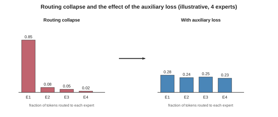
N = 4 experts

Balanced : f = [0.25, 0.25, 0.25, 0.25]   P = [0.25, 0.25, 0.25, 0.25]
           sum f*P = 4 * (0.25 * 0.25) = 0.25
           loss    = alpha * 4 * 0.25 = 1.0 * alpha      (the minimum)

Collapsed: f = [1.0, 0.0, 0.0, 0.0]       P = [0.7, 0.1, 0.1, 0.1]
           sum f*P = 1.0 * 0.7 = 0.7
           loss    = alpha * 4 * 0.7 = 2.8 * alpha      (penalized)
5. Interpreting Experts
AnalysisA natural guess is that each expert becomes a specialist in a subject, for example one for math, one for biology and one for code. To test this, the Mixtral paper colors every token of a text by the expert that processed it. The picture does not show a clear split by subject. Instead, the routing follows more superficial, syntactic patterns, such as the same expert handling certain keywords or indentation in code, and neighbouring tokens often going to the same expert. So "expert" here means a learned sub-network chosen by the router, not a human-style specialist, and the specialization is hard to describe in words.
Python code, one layer, colors = expert chosen for each token

class MoeLayer(nn.Module):        <- the tokens are spread over many colors
    def __init__(self, experts):  <- but the same token types (for example
        super().__init__()           "self" or indentation) tend to share
                                     an expert, regardless of topic
6. Predicting the Next Token with Sampling
DecodingAt the end of the Transformer, the softmax layer gives a probability for every word in the vocabulary, given the context \(C\) written so far. One option is to always take the single most likely word (greedy decoding), which is deterministic and often repetitive. The idea on the slide is to sample the next token from the whole distribution instead. Likely words are chosen more often, but unlikely ones can still appear, so the text becomes more varied. The chosen token is appended to the context and the process repeats for the next position.
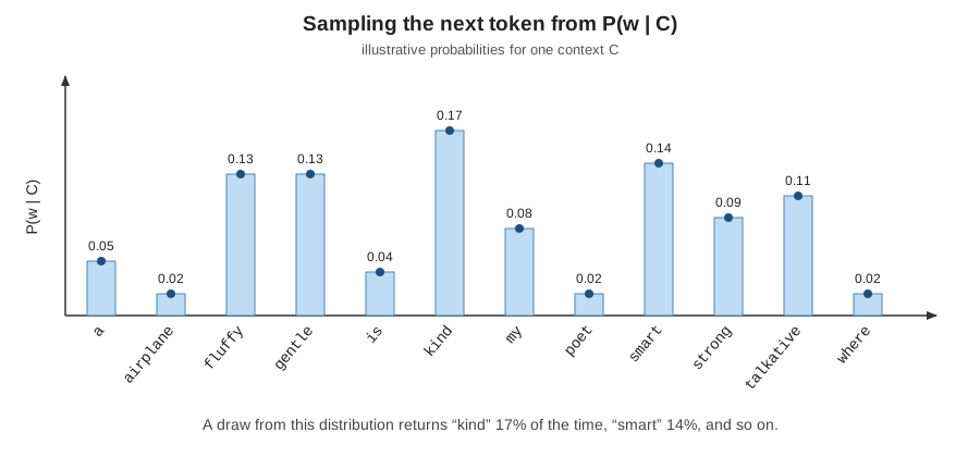
Context C = "My teddy bear is"            (probabilities are illustrative)

P(kind) = 0.17   P(smart) = 0.14   P(fluffy) = 0.13   P(gentle) = 0.13 ...

Greedy   : always "kind"
Sampling : "kind" about 17% of the time, "smart" about 14%, "fluffy" about 13%, ...
           so repeated runs can give different but sensible sentences
7. Constraining the Output via Guided Decoding
TechniqueSometimes a program, not a person, reads the model's answer, so the format must be exact. If you only ask the model for JSON in the prompt, it can still add extra text, forget a quote, or write a number as a word. Guided (constrained) decoding guarantees the format instead of hoping for it. At every step, a rule system decides which tokens could still lead to a valid output, the logits of all other tokens are set to \(-\infty\), the probabilities are renormalized, and the next token is sampled from what remains. The rules themselves are described with a finite state machine or a context-free grammar, covered next.
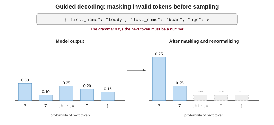
Prompt : "Generate a description of my 33-year old teddy bear who likes
          reading. Do this in JSON format."

Required output:
{
    "first_name": "teddy",
    "last_name": "bear",
    "age": 33,
    "hobby": "reading"
}

After  "age":  the rules allow only digits, so "thirty-three", a quote
or a closing brace are masked out and the model must write a number.
8. Finite State Machine (FSM)
Formal ToolA finite state machine is a small machine with a fixed number of states. It starts in a start state, reads symbols one at a time, and each symbol moves it along a transition to another state. If the input ends in an accepting state, it is valid. FSMs describe the same patterns as regular expressions, such as "one or more digits followed by a comma". For guided decoding, the generator keeps track of the current state: the tokens that have a transition out of that state are allowed, and the others are masked. After a token is chosen, the machine moves to the next state.
An FSM has only a fixed amount of memory (its current state), so it cannot count. It cannot check that braces are balanced to any depth, which is why nested structures need the more powerful tool in the next section.
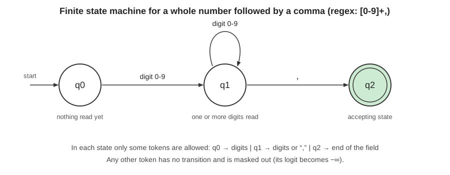
Pattern: one or more digits, then a comma     regex: [0-9]+,

Input "33,"  :  q0 --3--> q1 --3--> q1 --,--> q2   accepted
Input ",5"   :  q0 --,--> ?                        rejected (no transition)
Input "3a"   :  q0 --3--> q1 --a--> ?              rejected (no transition)

While generating after "age": the machine is in q0 (digits only);
after the first digit it is in q1 (digits or a comma).
9. Context-Free Grammar (CFG)
Formal ToolA context-free grammar describes a language with production rules. Each rule replaces one non-terminal (a named category such as Object or Value) with a sequence of non-terminals and terminals (actual characters or tokens such as "{" or ":"). It is called "context-free" because a rule can be applied to a non-terminal wherever it appears, whatever surrounds it. The key power of a CFG is recursion: a rule can refer back to itself, directly or indirectly, so it can describe nested structures of any depth, such as JSON objects inside objects, brackets in code, or nested parentheses.
To use a CFG in guided decoding, a parser follows the text generated so far and keeps a stack of what is still expected (for example, which braces are still open). From that state, it works out which tokens may come next and masks the rest. This can enforce a complete, valid JSON document, which an FSM cannot do on its own.
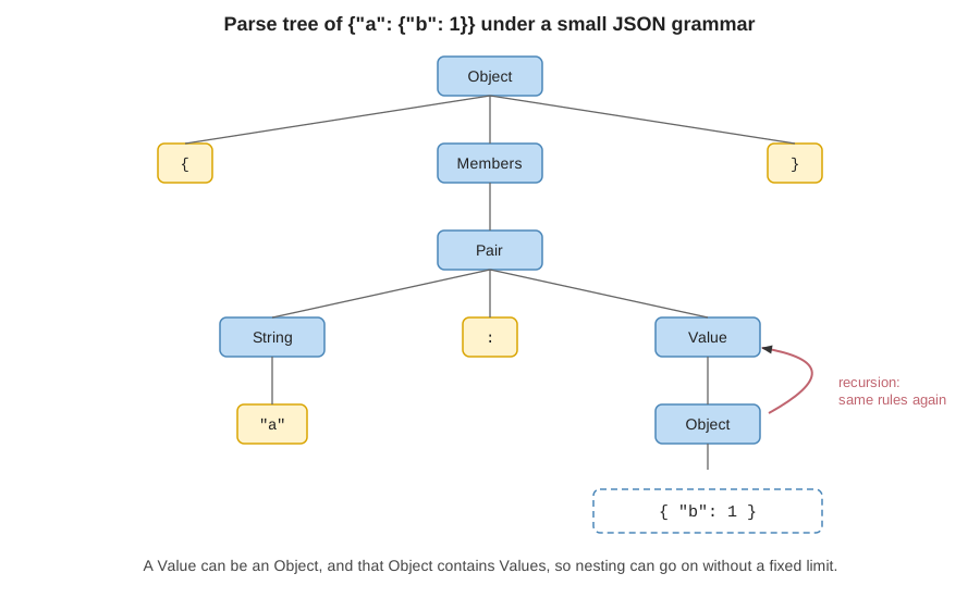
A small JSON grammar (non-terminals in capitals, terminals in quotes)

Object  -> "{" Members "}"
Members -> Pair | Pair "," Members
Pair    -> String ":" Value
Value   -> Number | String | Object        <- Object again: recursion
Number  -> Digit | Digit Number

Derivation of {"a": 1}:
Object => { Members } => { Pair } => { String : Value }
       => { "a" : Number } => { "a" : 1 }

During generation, after  {"first_name": "teddy",  the grammar expects
another Pair, so the next token must start a String (a quote).
A closing brace or a number would be masked out.
10. FSM vs CFG for Guided Decoding
Comparison| Aspect | Finite state machine | Context-free grammar |
|---|---|---|
| Describes | Regular patterns (regex) | Nested, recursive structures |
| Memory | Only the current state | Current state plus a stack |
| Can it match nested brackets? | No (depth is unbounded) | Yes |
| Typical use | Numbers, dates, IDs, fixed choices | Full JSON, code, expressions |
| Cost | Cheap and simple | More complex to run |
Field value "age": 33          -> an FSM is enough ([0-9]+)
Whole document with nesting    -> needs a CFG:
{ "pet": { "name": "teddy", "toys": { "book": 1 } } }

Both work the same way inside the decoder:
state -> allowed tokens -> mask the rest -> sample -> new state